Chapter 2 Data Description
2.1 Green Space Data
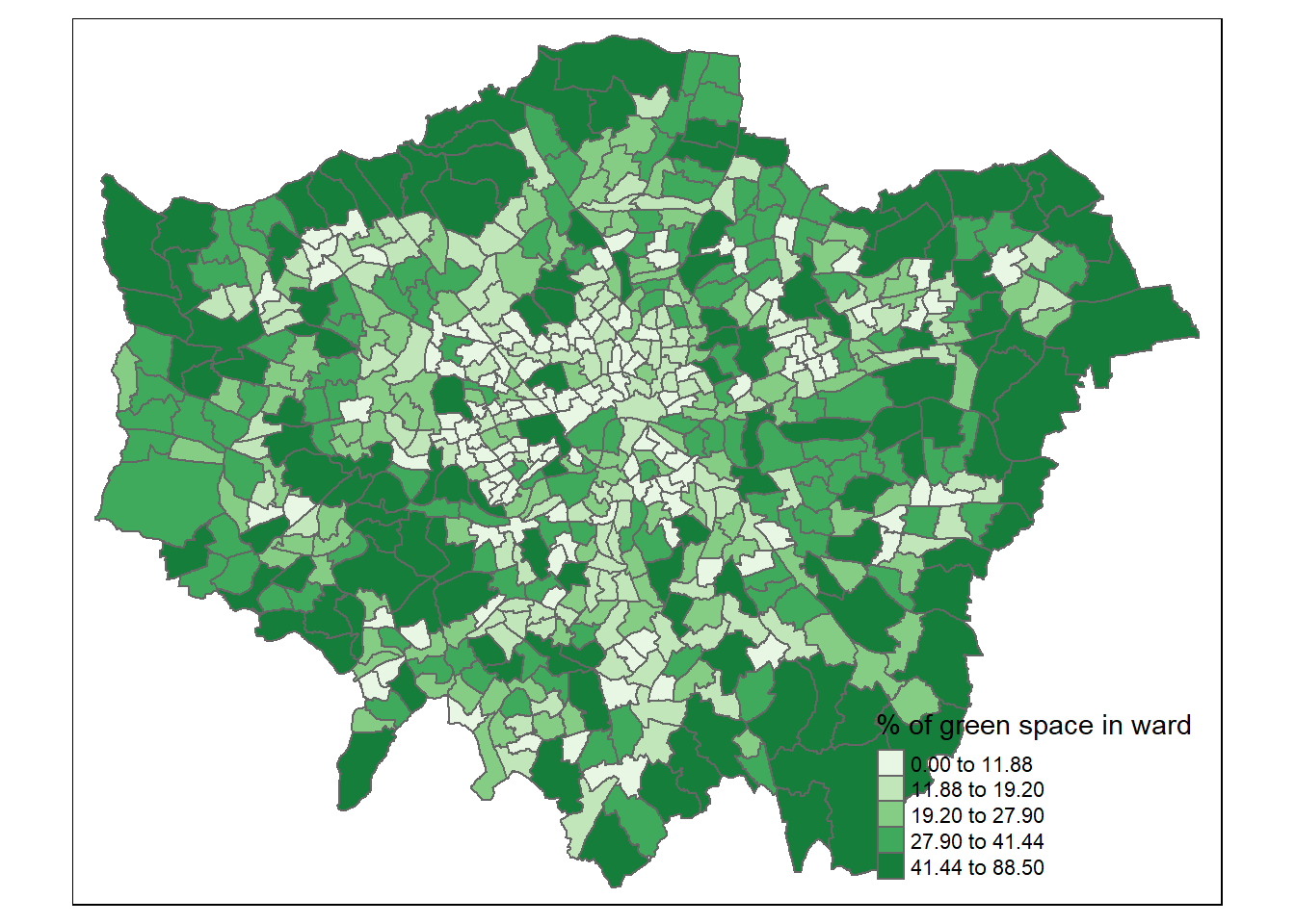
There are a number of ways to measure access to green space, each with their own limitations. For this study, the percentage of ward land area used for green space was taken as a proxy for access to green space for residents in that ward. The limitations of this proxy are discussed in detail later in this report. The data for this proxy was sourced from Ministry of Housing (2005). This is part of the Generalised Land Use Database published by the Ministry of Housing, Communities & Local Government (MHCLG) in 2005. The dataset includes two forms of data: the land area of each London ward and the percentage of this area used for each possible land use. A clear pattern in the spatial distribution (Figure 2.1) of this data is the greater percentage of green space per ward in the ‘Green-Belt’ of suburban London (a statutory ring of green areas surrounding the capital). This is particularly clear in East and West London.

Figure 2.1: % of green space per ward in Greater London

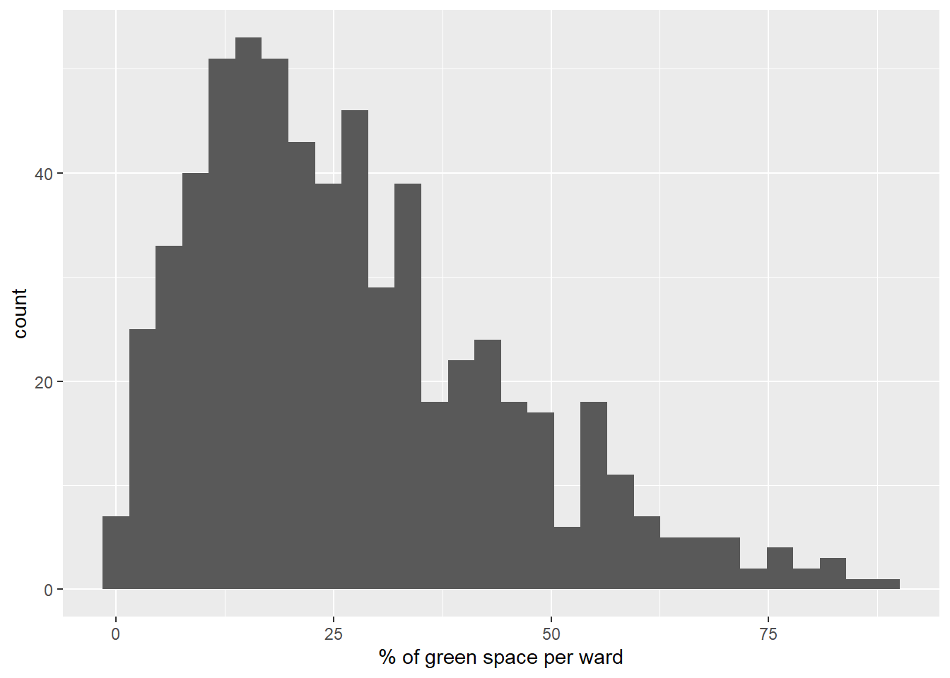
Figure 2.2: Histogram of % of green space per ward in Greater London
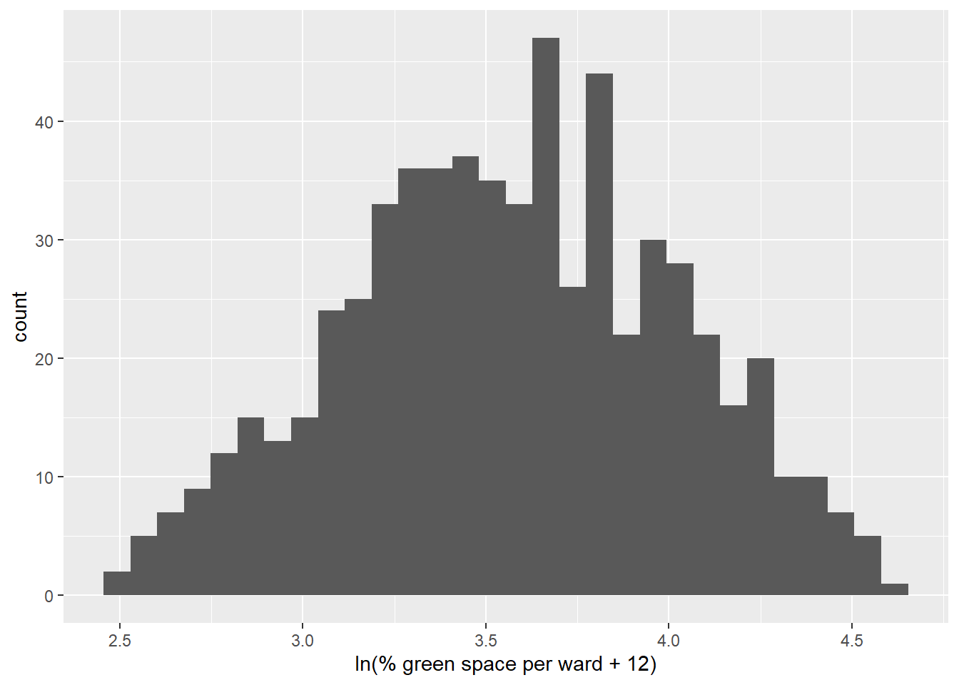
Figure 2.2 shows that the data is not normally distributed, which could reduce the integrity of our models. The data can be normalised by taking the natural logarithm of the percentage of the area used after finding the sum of twelve and the variable (ln(green space + 12)). The result is shown in Figure 2.3.

Figure 2.3: Histogram of normalised % of green space per ward in Greater London
It is important to note the limitation of the measure of access to green space used in this study, particularly the lack of consideration of network access, or access to green space in neighbouring wards. A number of datasets were considered for the study. A possible choice was a dataset Access to Public Open Space and Nature (Greater London CIC (GiGL) (2015)). This dataset contains the percentage of residential households per ward that have sufficient access to green space in line with UK governmental standards (London (2017)). However, this data was found to be extremely skewed, which made it impossible to define an appropriate model. After analysis of a number of other data sources, the source used in this study was decided to be most appropriate.
2.2 Demographic Data
After a literature review, a shortlist was created containing independent variables likely to be significantly correlated with access to green space. These were all aggregate statistics for wards including average income, average age, ethnicity, average wellbeing and average life expectancy. The data for these variables was sourced from the UK 2011 Census dataset (National Statistics (2011)). The UK Office for National Statistics provided a rigorous data collection system to capture the data on the questionnaires, interpret it and confirm it, making the census data trustworthy and reliable. As the data for these variables share a source, they are consistent in time. However, since these data were collected ten years ago, they may no longer be representative. The census data required refining and cleaning before use. Unnecessary data was removed and the data was examined for null values. The data was then compiled in a comma separated values file for use in R. This file was joined to a shapefile of London ward boundaries, producing a shapefile containing geographic boundaries, demographic and health information. The following variables required transformation with a natural logarithm in order to fit a normal distribution: number of Black people in the ward, number of Asian people in the ward, average income of the ward, number of people of ‘Other’ ethnicity.
2.3 Data Multicollinearity
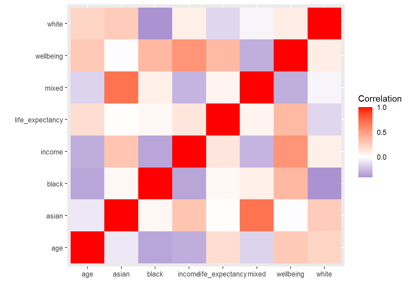
Multicollinearity refers to the precise correlation or high correlation between explanatory variables in the linear regression model (Daoud (2017)). Multicollinearity between independent variables may significantly reduce the regression model’s fit. Figure 2.4 and Table 2.1 show the correlation between independent variables, and the VIF values for independent variables, respectively.

Figure 2.4: Correlation matrix for dependent variables.
| Independent variable | VIF |
|---|---|
| age | 2.628899 |
| life expectancy | 2.142507 |
| income | 2.971197 |
| asian | 1.779267 |
| black | 6.177844 |
| mixed | 3.613875 |
| other | 2.365799 |
The results of tests for multicollinearity revealed high correlations between a number of the independent variables. In general, the correlation coefficient between 0 and 0.5 means that the model is less likely to have multicollinearity problems, while the correlation coefficient between 0.5 and 1 means that the model may have serious multicollinearity problems. If the VIF is greater than 5, there could be obvious multicollinearity in the model (Daoud (2017)). Combined with these two parameters, the data of wellbeing and white ethnicity were removed to reduce the multicollinearity.