Chapter 5 Results
Base Formula: \[\large ln (g + 12) = age + le + ln(income) \\ \large + ln(ap/tp) + ln(bp/tp) + (mp/tp) + ln(op/tp)\]
\(\Large g\) = % green space in ward
\(\Large age\) = mean age in ward
\(\Large le\) = life expectancy in ward
\(\Large income\) = mean income in ward
\(\Large tp\) = total population in ward
\(\Large ap\) = asian population in ward
\(\Large bp\) = black population in ward
\(\Large mp\) = mixed ethnicity population in ward
\(\Large op\) = population in ward of ethnicities other than white or those previously stated
Spatial Durbin, Error and Lag models for each respective study area used the same base formula, predictive variable, dependent variable, and spatial weight matrix (first-order queen criterion) as above. The wards immediately adjacent were considered neighbours whether they touched the corners or the flat edge of a ward’s polygon. An identical strategy was used in the GWR model though varied by selecting a relevant bandwidth for the isotropic Gaussian Kernel. In this study, when a result is deemed statistically significant, it will refer to a p-values ≥0.05, correspondingly <0.05 is not significant.
5.1 OLS
The Ordinary Least Squares (OLS) models fitted to each region were significant (at the 95% level) and returned an adjusted R2 0.1052-0.2722, West London returning the highest result. The OLS models only explained 10-27% of the green space variation for each location. Combined with the High Residual Standard Error (RSE) 0.3804 – 0.4365, it can be concluded that OLS was a poor fit for modelling green space both in the subdivisions and the whole of London. This can be observed in the large difference between the actual value of green space and the predicted value.
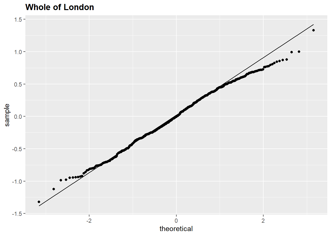
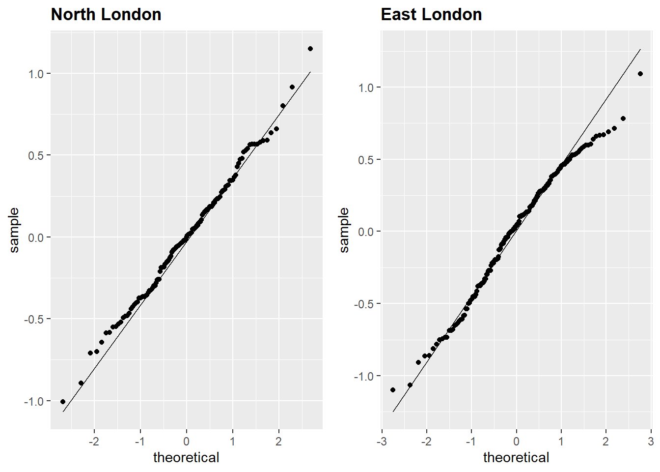
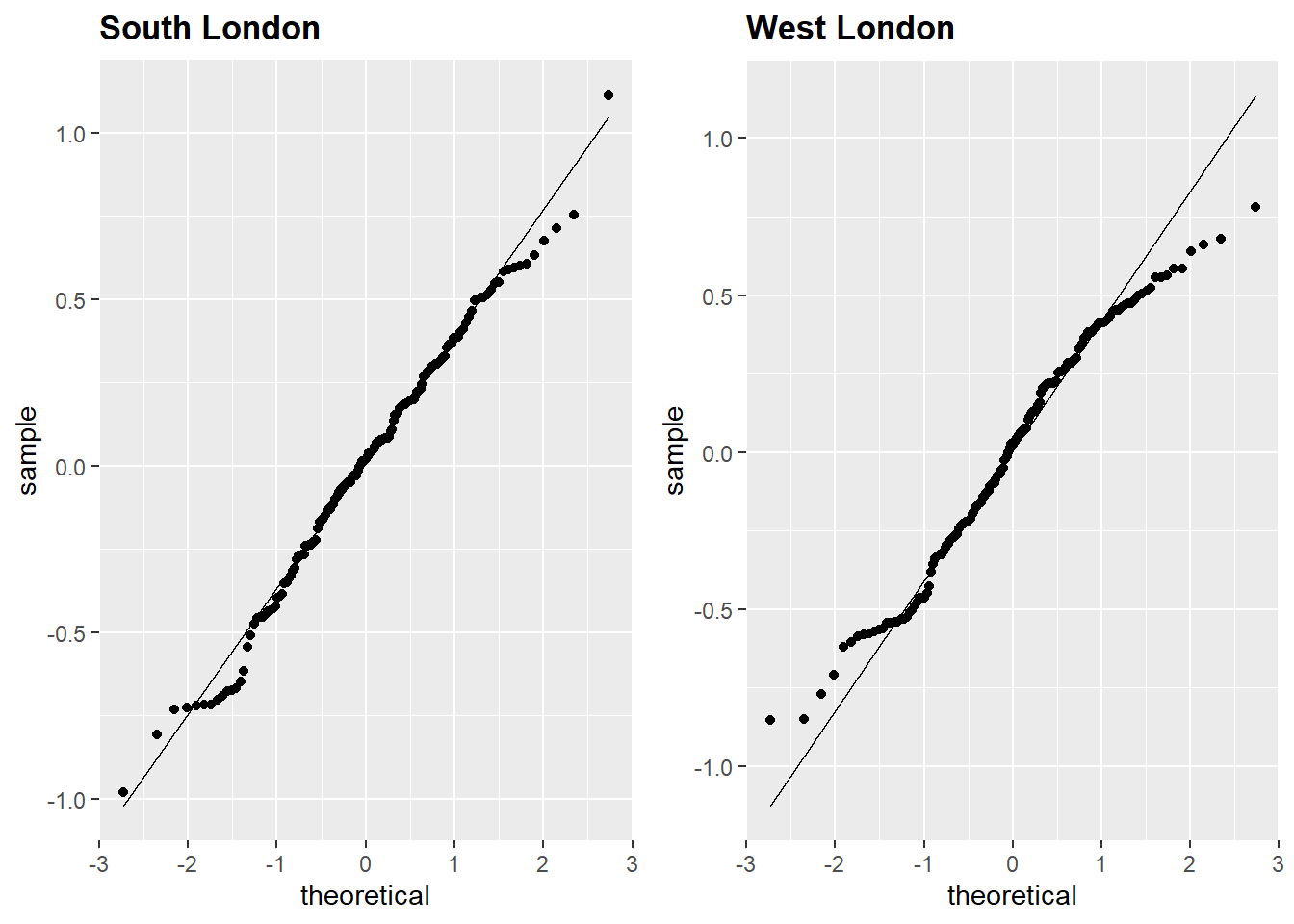
Figures 5.2, 5.3 and 5.1 display the Q-Q plots for all datasets. All plots showed that points were above the theoretical normal line at the lower values near the beginning and below the line near the end. The plots exhibited a thin-tailed distribution; deviation at the ends was considered negligible. Consequently, the datasets were considered close to normal distribution: the Shapiro-Wilk test provided further evidence of normality.

Figure 5.1: Q-Q plot of linear model residuals, Greater London

Figure 5.2: Q-Q plot of linear model residuals, North London and East London

Figure 5.3: Q-Q plot of linear model residuals, South London and West London
5.2 Shapiro-Wilk Normality Test
The Shapiro-Wilk (Shapiro and Wilk (1965)) results for the OLS residuals for North, East and South areas were not significant at a 95% confidence level (p-value > 0.05) and had a high W value. Thus, the null hypothesis of a normal distribution was not rejected, and normality in the residuals was assumed. Conversely, London as a whole and the West were weakly significant at a p-value of 0.02431 and 0.00907. For this study these values were deemed acceptable enough for the assumption of normality. Similarly, the natural logarithm transformation and addition of 12 to the dependent variable showed a significant increase in assumed normality.
5.3 Moran’s I on OLS residuals
The Global Moran’s I test results on the OLS residuals detected statistically significant and positive spatial autocorrelation; similar green space values were clustered together in all areas apart from the South (Table 5.1). The whole of London and the West had the largest Moran’s I of 0.171590363 and 0.177676307 and a p-value 5.826E-15 and 2.65E-06. The results stated that, with the exception of the South, the null hypothesis of spatial randomness could be rejected with confidence. The results also suggested that the unaccounted spatial autocorrelation in the OLS residuals was a key factor causing the high RSE and low R2 value.
| London | North | East | West | South | ||
|---|---|---|---|---|---|---|
| 1 | Observed Moran’s I | 0.1715903627 | 0.087117028 | 0.108292348 | 0.177676307 | -0.03053761 |
| 2 | Expectation | -0.0083988916 | -0.0352447 | -0.025650785 | -0.030140504 | -0.03025517 |
| 3 | p-value | 5.826E-15 | 0.007698 | 0.001336 | 2.65E-06 | 0.5023 |
5.3.1 South
Contrary to all other results, the South had a negative observed Moran’s I -0.03053761 nearly identical to the expectation value of -0.03025517: the value if no spatial autocorrelation was present. The Moran’s I value when combined with the statistical insignificance, indicated that there was not enough evidence to suggest that spatial autocorrelation was present. The fitting of a spatial regression model would not improve the prediction of green space, therefore, despite its limitations, the OLS model was concluded to be the best fit available for South London.
5.4 Lagrange Multiplier Tests
Table 5.2 shows all the Lagrange Multiplier test results.
| London | North | East | West | South | ||
|---|---|---|---|---|---|---|
| 1 | LMlag | 56.262 | 7.5719 | 7.2718 | 1.85E+01 | 0.96829 |
| 2 | p-value (LMlag) | 6.34E-14 | 0.005928 | 0.007005 | 1.73E-05 | 0.3251 |
| 3 | LMerr | 52.139 | 2.5679 | 5.2787 | 13.204 | 0.36006 |
| 4 | p-value (LMerr) | 5.17E-13 | 0.1091 | 0.02159 | 0.0002793 | 0.5485 |
| 5 | RLMlag | 4.1866 | 11.009 | 3.1031 | 6.2264 | 2.7989 |
| 6 | p-value (RLMlag) | 0.04074 | 0.0009069 | 0.07814 | 0.01259 | 0.09433 |
| 7 | RLMerr | 0.063807 | 6.0046 | 1.11 | 0.96381 | 2.1907 |
| 8 | p-value (RLMerr) | 0.8006 | 0.01427 | 0.2921 | 0.3262 | 0.1388 |
5.4.1 London
For London as a whole the LMerr and LMlag values were high, 56.262 and 52.139, and significant at a 95% confidence. However, the robust test indicated a Spatial Lag model should be fitted as the RLMerr was low and insignificant.
5.4.2 North
Likewise, for the North, the results indicated that a Spatial Lag model would best fit the data. The LMlag value was significant, whereas the LMerr was not, the robust test produced similar results.
5.4.3 East and West
The East and West demonstrated statistical significance for both regular LM tests. However, the robust test for RLMerr values was lower than LMlag and not significant for the West, signifying that a Spatial Lag model should be fitted. In contrast, both robust LM tests for the East had a p-value > 0.05; both Error and Lag would be run.
5.4.4 South
Both LM tests was insignificant for South London, this was expected considering the Moran’s I result concluded that there was not enough statistical evidence to stipulate the presence of autocorrelation.
5.5 Spatial Regression Models
The LM test and Global Moran’s I guided the procedure for model testing and selection. Even with this guidance, all models for each study area and dataset were run to provide supporting evidence for model selection and highlight a model’s unsuitability.
5.5.1 Spatial Lag Model
The Spatial Lag model’s Rho value ranged from 0.29468-0.45669 with significant p-values for London, North, East and West. The results imply that there was a lagged relationship between green space values in neighbouring wards. The spatial autocorrelation detected in the Moran’s I was modelled out for all three locations; the p-value exceeded the 0.05 threshold. Therefore, the null hypothesis of spatial randomness could not be rejected.
Compared to the OLS, the AIC of the Lag model demonstrated a distinct decrease, across all study regions: the whole of London showed the most considerable change 695.5 to 648.57. The reduction signified the model’s better fit for predicting green space values. The Rho and residual autocorrelation test’s lack of statistical significance in the South was reflected in the increased AIC, from 159.21 to 160.9, this was interpreted as the worst fit.
5.5.2 Spatial Error Model
The LM test results suggest that only the East dataset be modelled with the Spatial Error; despite this, all datasets were passed through each model and tested to allow for complete comparison. The Spatial Lag’s unique coefficient, lambda, had a high value and was statistically significant in all regions apart from the North and South; which highlighted potential clustering in the residuals. Nevertheless, the log-likelihood was more negative; also the AIC was higher than the Spatial Lag results. The Akaike Information Criteria rule of thumb states that if the AIC value of models falls within two or less, they have the same explanatory power (Fabozzi et al. 2014). None of the Spatial Errors results fell within the parameter; for that reason, the model was deemed a less adequate fit relative than the Lag.
5.5.3 Spatial Durbin
The Rho values for the Durbin model in the North was not significant at a 95% confidence level. The reduced AIC and less negative Log-likelihood for the London dataset provided evidence that Durbin model would be a better fit than the Lag. The AIC of the East had a difference greater than two in comparison to the Lag; therefore, the model was interpreted as weaker in explaining power. Across all study areas, spatial autocorrelation had been modelled out similar to the Lag. In the results for the West, conflict arose between the Log-likelihood and AIC value between the Durbin and Lag model. Durbin had a greater AIC 143.31 and less negative log-likelihood -54.65 compared to 137.71 and -58.85 of the Lag. Despite the contradiction, Lag was interpreted as the best fit, based on the principle that AIC was used as the primary model selection parameter. When similar conflicts arose throughout the study, the same approach was taken.
5.5.4 GWR
The spatial autocorrelation evident in the OLS model’s residuals was reduced in all study areas in which the GWR model was run, though not wholly modelled out. Excluding the South, the observed Moran’s I ranged 0.087117-0.177676 (OLS residuals) compared to 0.0175191-0.08093797 (GWR) all with an associated p-value < 0.05. In accordance with the reduction in observed spatial autocorrelation, the AIC for all study regions was considerably lower for GWR than the OLS, Lag, Durbin and Error models. The R2 value significantly increased across all areas when compared to the OLS.
5.5.5 OLS and Spatial Filtering
The OLS model is nested within the OLS and Spatial Filtering model, hence comparison of their results represents the direct impact of Spatial Filtering function upon the model’s strength .Apart from the South, every study area observed a noticeable decrease in RSE 0.3804-0.4365 to 0.3218-0.4047 compared to the initial OLS results. The adjusted R2 rose considerably from 0.1286-0.2722 to 0.2922-0.4791.
The transition of the results demonstrated how each model’s predictive power increases with spatial autocorrelation being modelled out; the Global Moran’s I was statistically insignificant in each study area. Across London, East, West and North the AIC was the smallest when compared to the OLS, Lag, Durbin and Error models. However, in all areas apart from Greater London GWR had a lower AIC. There was a difference in AIC value less than one for Greater London. According to Akaike Information Criteria rule of thumb, the minor difference indicates that the two models have the same explanatory power (Fabozzi et al. 2014).
The full list of AIC values for each model is displayed in Table 5.3. The GWR model for all areas, including the South, had the smallest AIC value overall. This was closely followed by OLS and Spatial Filtering, then the Lag model. Despite the lower GWR AIC avlue, OLS with Spatial Filtering was concluded to be the best fit in all areas except the South. This is due to the limitations of the GWR, most notably the inability of GWR to remove spatial autocorrelation in residuals. The OLS with Spatial Filtering model was the only model to fully remove spatial autocoreelaiton in residuals. Excluding the North and South, the Durbin model for the other locations had the fourth-highest AIC. All results, not including the South, indicated Error being the second least powerful spatial regression model. Finally, the OLS was the model deemed weakest at providing accurate predictive greenspace values.
Full results for all models are available in the Appendix.
| London | North | East | West | South | ||
|---|---|---|---|---|---|---|
| 1 | Number of Observations: | 625 | 135 | 173 | 159 | 158 |
| 2 | OLS | 695.9519 | 134.9908 | 213.9736 | 153.6169 | 159.2142 |
| 3 | Error | 650.3795 | 133.7242 | 210.6101 | 141.3932 | 160.7782 |
| 4 | Lag | 648.5731 | 129.6145 | 208.956 | 137.711 | 160.0925 |
| 5 | Durbin | 639.2799 | 131.1229 | 213.5265 | 143.3125 | 165.3068 |
| 6 | GWR | 564.501 | 98.46093 | 196.742 | 93.19053 | 144.7065 |
| 7 | OLS and Spatial Filtering | 564.4889 | 118.6283 | 192.471 | 110.4278 | 159.4238 |