Chapter 6 Discussion and Conclusions

6.1 Model Selection

For most of the study areas, it is evident that a spatial regression model is necessary to account for the spatial autocorrelation and reduce errors. The principle of model selection based solely on AIC is useful but not entirely sufficient. Geographically Weighted Regression has the lowest AIC in every area apart from London (whole) and the South, indicating the best fit. However, for models in all areas there remains statistically significant spatial autocorrelation in the residuals. The Ordinary Least Squares with Spatial Filtering was the only model remove this autocorrelation, reducing the model’s error and increasing its explaining power. For this reason, Ordinary Least Squares and Spatial Filtering were chosen as the best model for predicting green space in all areas where spatial autocorrelation was observed (i.e. all areas except South London).

Below are details of the models selected as most appropriate for each area. Figures 6.1, 6.2, 6.3, 6.4 and 6.5 display side by side choropleths of London, North, East, West and South. The left map represents the dataset’s values for the percentage of green space; the map adjacent shows fitted or predicted values for the most appropriate model for the area.

\(\large g\) = % green space in ward
\(\large age\) = mean age in ward
\(\large le\) = life expectancy in ward
\(\large income\) = mean income in ward
\(\large tp\) = total population in ward
\(\large ap\) = asian population in ward
\(\large bp\) = black population in ward
\(\large mp\) = mixed ethnicity population in ward
\(\large op\) = population in ward of ethnicities other than white or those previously stated
\(\large spatial filter\) = fitted result of Roger Bivand’s semi-parametric spatial filtering function (Bivand (2007)) applied to the Ordinary Least Squares model for the area. Documentation for the spatial filtering function can be found at https://www.rdocumentation.org/packages/spatialreg/versions/1.1-5/topics/SpatialFiltering.
\(\large VC\) = coefficients for the vectors of the spatial filter, as shown in Appendix Section 7.6.

6.1.1 Greater London

Ordinary Least Squares with Spatial Filtering

\[\large g = exp(0.0297(age) -0.0028(le)\\ \large -0.5967(ln(income)) -0.0341(ln(ap/tp)) \\ \large-0.0271(ln(bp/tp)) -0.0001(mp/tp) -0.0498(ln(op/tp)) \\ \large + VC(fitted(spatial filter))) -2.129 \]

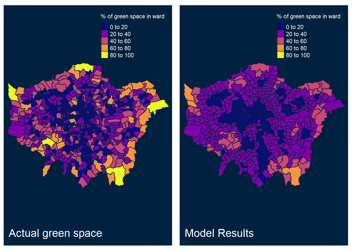
Figure 6.1: Fitted and observed values of % green space per ward in Greater London

6.1.2 North London

Ordinary Least Squares with Spatial Filtering

\[ \large g = exp(0.0724(age) + 0.0474(le) \\ \large -0.1172(ln(income)) - 0.0008(ln(ap/tp)) \\ \large + 0.4206(ln(bp/tp)) -0.0650(mp/tp) -0.0498(ln(op/tp)) - 3.7756\\ \large + VC(spatial filter)) - 12 \]

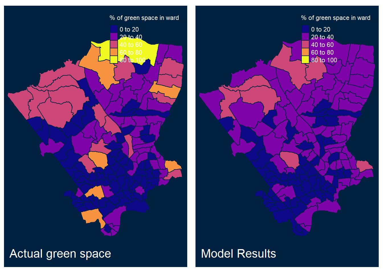
Figure 6.2: Fitted and observed values of % green space per ward in North London

6.1.3 East London

Ordinary Least Squares with Spatial Filtering

\[ \large g = exp(0.0119(age) -0.0252(le) \\ \large -0.1075(ln(income)) -0.1683(ln(ap/tp)) \\ \large + 0.0236(ln(bp/tp)) + 0.0005(mp/tp) -0.0860(ln(op/tp))\\ \large + 7.7045 + VC(spatial filter)) -12 \]

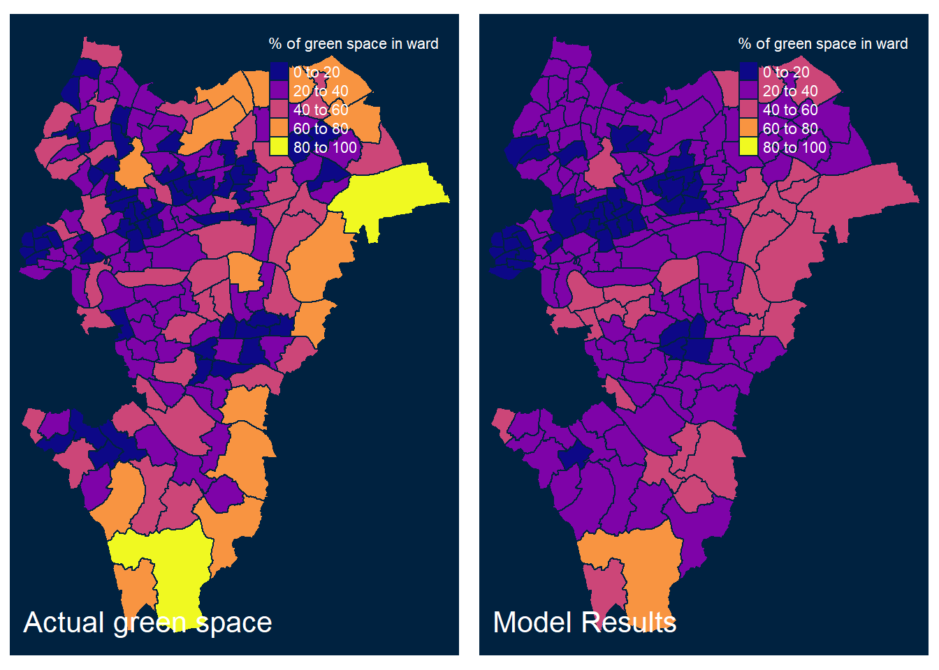
Figure 6.3: Fitted and observed values of % green space per ward in East London

6.1.4 West London

Ordinary Least Squares with Spatial Filtering

\[ \large g = exp(0.0504(age) -0.0168(le) \\ \large -1.4774(ln(income)) + 0.0137(ln(ap/tp)) \\ \large -0.3282(ln(bp/tp)) + 0.0003(mp/tp) -0.0110(ln(op/tp))\\ \large + 20.8318 + VC(spatial filter)) -12 \]

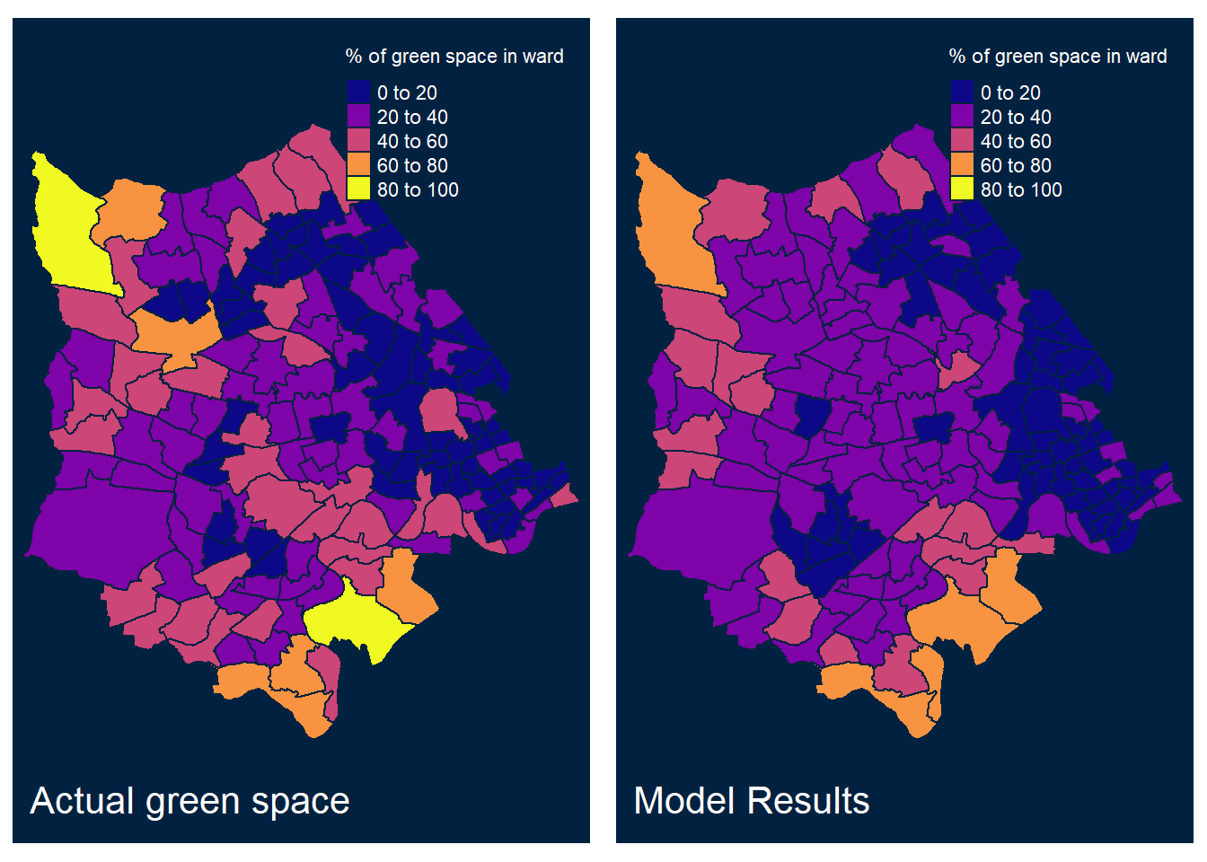
Figure 6.4: Fitted and observed values of % green space per ward in West London

6.1.5 South London

Ordinary Least Squares

\[\large g = exp(0.0122(age) + 0.0155(le) \\ \large -0.3715(ln(income)) -0.0415(ln(ap/tp)) \\ \large + 0.0263(ln(bp/tp)) -0.0002(mp/tp) -0.1623(ln(op/tp)) + 6.9080) -12 \]

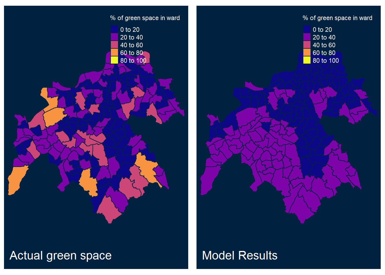
Figure 6.5: Fitted and observed values of % green space per ward in South London

It can be seen that these models are fairly competent for predicting the spatial distribution of access to green space, but underestimate values in the vast majority of cases. It can be concluded that the independent variables considered in this study are somewhat reliable predictors of access to green space, and therefore are closely related. The sign and magnitude of coefficients in the models can be interrogated to understand the relative influence different independent variables have on predicting access to green space in a ward. For example, in most of the models the number of Mixed ethnicity people living in the ward has less influence on predicting access to green space than the median age of the residents of that ward, as demonstrated by the relative magnitudes of their coefficients. The coefficient for the median age variable is positive in all models, suggesting wards with an older population have better access to green spaces. A number of the independent variables have coefficients of different signs in models of different areas, highlighting the importance of modelling at a local scale rather than assuming a pattern in one area will be replicated elsewhere. The requirement of different models for different areas emphasises the complexity of access to green space, further work may create a more robust model that fits data for all the study areas.

6.2 Limitations and future work

Significant multicollinearity between independent variables raises concerns for the results of this study. Regression analysis assumes that a change in the value of an independent variable should change the value of the dependent variable and not affect any other independent variables (Farrar and Glauber (1967)). However, correlation between independent variables (multicollinearity) reduces the precision of coefficient estimates, which in turn reduces the reliability of p-values and increases the difficulty of identifying statistically significant independent variables. It can also cause coefficient estimates to change dramatically if small changes are made to other independent variables in the model (Farrar and Glauber (1967)). Two approaches were considered to reduce multicollinearity. The first approach would be to combine highly correlated independent variables into larger categories; however, this was considered to be an oversimplification and inappropriate considering the nature of the variables involved. The second approach would be to remove highly correlated variables. As the ‘wellbeing’ variable showed a high correlation with many other independent variables it was removed. The ‘white’ variable was also highly correlated with many other independent variables and had much higher values in each ward than other ethnic groups. Therefore, this variable was also removed. Future work could seek to further reduce correlations between independent variables or create a model unlikely to be influenced by multicollinearity.

A variety of indicators were available for evaluating model fit including log-likelihood, R², spatial tests on regression residuals, Lagrange-Multiplier tests, Alkaline Information Criterion, Bayesian Information Criterion and least squares. The Alkaline Information Criterion proved easiest for comparison between models as this indicator was available when using regression functions from the R packages ‘spdep,’ ‘spgwr’ and ‘spatialreg.’ However, other indicators showed different relative best fit between models. Future work could further evaluate the fit of each model in greater detail, and interrogate the merits of each measure of model fit in greater depth.

This study uses the aggregated spatial units of London wards (official subdivisions of London boroughs). These units were used because they are a well-understood subdivision of London and relevant to those working for London councils or planners, the key stakeholders in this study. Wards are the finest spatial units available for the London data required and are standardised across all of the datarequired for this study. Two problems are introduced due to the aggregation of spatial point data into areal units: the modifiable areal unit problem (MAUP) and the problem of ecological fallacy. The MAUP occurs because the results of statistical analysis can change significantly depending on the size, shape and position of the aggregated areal units used (Goodchild (2011)). The aggregated value will be generated using different point values depending on these three factors. The problem of ecological fallacy occurs when assumptions are made about individual locations or people within a ward based on the characteristics of that ward as a whole (Goodchild (2011)). Large differences in the size of areal units can lead to heteroskedasticity in the residuals from regression analysis. The weight matrix used for spatial regression analysis can also significantly affect the results, for example, this study uses a Queen’s weight matrix. This matrix yields different results to a Rook’s matrix. Further work could seek to evaluate the most appropriate matrix in greater depth.

There are a number of ways to measure access to green space, each with their own limitations. Perhaps the most reliable measure is to use walkable network distance from each individual home in an area to the nearest entrance to a green space (Greenspace Information for Greater London (2015)). A similar measure was used for a case study of Leicester, the measure was the same except for the use of centres of population census output areas in place of individual homes (Comber, Brunsdon, and Green (2008)). Many planning authorities simply use Euclidean distances from homes to green spaces to measure access (Moseley et al. (2013)). Other studies have used the percentage land use vs. population in an areal unit (Barbosa et al. (2007)). Our study first attempted to use the GIGL dataset for regression analysis, however, the residuals of regression analysis were extremely skewed. Normally distributed residuals are desired for regression analysis (Jarque and Bera (1987)), therefore this dataset was considered inappropriate for our study. Various other datasets and measures were tested for normality of regression residuals, including Euclidean distance to green space for and metric area of green space divided by population per ward. The only data to give normally distributed residuals was a measure of percentage area of green space per ward. Therefore, this data was used for our regression analysis despite the noted lack of nuance in the measure. The data does not consider access to green space across ward boundaries, network walking distances, equality of distribution of green space within a ward or quality of green space. Further work could produce or source a dataset appropriate for regression analysis that considers these important factors.