Chapter 4 Methodology

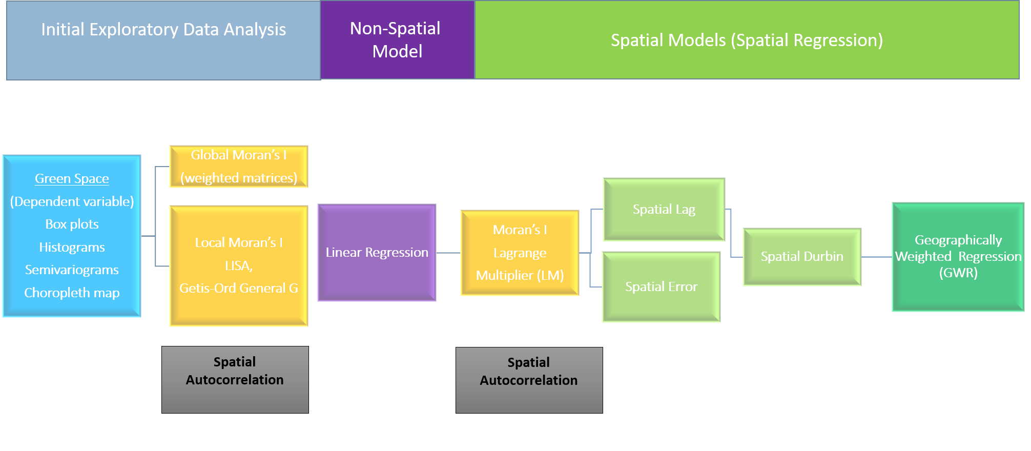
Figure 4.1 The analyse, evaluate, decision-making approach used for our study.

A literature review was completed in order to gain domain knowledge for the study, establish gaps in the literature and understand the methods used by other researchers for analysing variations in access to green space. From this appropriate methods and variables were established. Data was sourced with careful consideration to reliability and completeness. Exploratory analysis was performed on this data, and variables were normalised where required. Tests for local and global spatial autocorrelation were performed to establish whether spatial regression models would be required; these included Global and Local Moran’s I, and Getis and Ord’s Gi and Gi*. Spatial autocorrelation can be described as the extent to which attributes of objects are significantly clustered spatially, which can result in the possibility of underestimating errors and overestimating the statistical significance of regression coefficients in a model (Haining (2003)). Testing and modelling were performed on Greater London and sub-sections of London to understand variation in results in different areas and at different scales.

An Ordinary Least Squares (OLS) multiple linear regression model was the first model created. The residuals of this model were examined for spatial autocorrelation using Lagrange Multiplier tests and Moran’s I. The results of these tests guided the procedure for model testing and selection. After each stage of modelling the results were analysed and evaluated before deciding whether further modelling was required, this procedure is illustrated in Figure 4.1. Even with this guidance, all models for each study area and dataset were run to provide supporting evidence for model selection and highlight a model’s unsuitability. The spatial models were tested in the order Spatial Lag, Spatial Error, Spatial Durbin, Geographically Weighted Regression, OLS with Spatial Filtering. Finally, the most suitable model for each study area was chosen.

The spatial lag model takes significant autocorrelation in the dependent variable as the assumption but may also take varying spatial scales in the data into account (Chi and Zhu (2008)). On the contrary, the spatial error model suggests spatial autocorrelation in errors, as a result of key independent variables that have not been included in the model. The third spatial regression model used was the Spatial Durbin model, which implies that autocorrelation may be present in one or more independent variables, as well as the dependent variable. A Geographically Weighted Regression (GWR) model allows for the model to vary over space, by passing a search window from a multitude of points in the study area and fitting a distance weighted regression model each time (Brunsdon (2008)). A benefit of the GWR over more basic spatial regression models is that it accounts for spatial heterogeneity, which can be particularly important to represent parts of London that are on the boundaries of wards, for example.

The OLS with Spatial Filtering model uses Eigenvector Spatial Filtering Regression (ESFR) to explain the underlying spatial processes in the regression model and account for the autocorrelation present. The spatial filter is included into the OLS regression model to represent spatial autocorrelation as a synthetic variable obtained from a linear combination of selected spatial weight matrix eigenvectors (Griffith and Paelinck (2011)). The eigenvectors in a linear format allow for the filtering of spatial autocorrelation in the regression residuals, as well as increased model accuracy and reduced uncertainty as each eigenvector is uncorrelated with each other (Getis and Griffith (2002)).

The study was completed using the R programming language within the RStudio application, enabling the incorporation of tools to compute our results and display them in graphical form. The codes used have been stored for reproducibility.